ProofWatch

I’ll discuss my first arxived research as a PhD student in language more fitting for a layperson. I’m glad to have had the opportunittty to collaborate with the good, senior researchers on ProofWatch.

(My technical first publication, The global brain and the emerging economy of abundance: Mutualism, open collaboration, exchange networks and the automated commons, is purely conceptual. Now my hands have been dirtied.)

If the abstract doesn’t look like a foreign tongue to you, just go read the paper :). (And you may want to skip to the end and look at the shiny plots and brief commentary not found in the paper.)

ATP and ITP Background

My research is in the field of Automatic Theorem Proving and Interactive Theorem Proving.

Everyone knows that \((-1)\times(-1) = 1 \). So let’s look at an example theorem using \(a\) and \(b\) instead of 1 because they make algebra more clear.

Theorem: \((a \times b) = (-a) \times (-b)\)

Below I’ll use \(ab \mathsf(:-) a \times b\) because it’s clearer.

Let’s write down some things we know about arithmetic. Part of what we call our “Background Theory”.

1. Additive Identity: \(z + 0 = z\)
2. Addiditve Inverse: \(a + (-a) = 0\)
3. Distributivity: \(a(b+c) = ab + ac\)
4. Commutativtiy: \(a + b = b + a\) and \(ab = ba\)
5. Zero Product Property (Theorem): \(z0 = 0\)

These are our premises and we can use them to prove our theorem. Premises 1-4 are axioms, that is they are fundamental parts of our definition of arithmetic (ok, of Fields). Premise 5 is a prior theorem, one we already proved from the axioms (and maybe other theorems, or lemmas (mini-theorems or intermediate-theorems). When we think something is true, a Theorem, but haven’t proven it yet, we call it a conjecture.

1. \(ab = ab\)
2. \(ab = ab + 0\) by Additive Identity
3. \(ab = ab + (-a)0\) by Zero Product Property
4. \(ab = ab + (-a)(b + (-b))\) by Additive Inverse
5. \(ab = ab + (-a)b + (-a)(-b)\) by Distributivity
6. \(ab = (a + (-a)b + (-a)(-b)\) by Distributivity
7. \(ab = 0b + (-a)(-b)\) by Additive Inverse
8. \(ab = 0 + (-a)(-b)\) by Zero Product Property
9. \(ab = (-a)(-b)\) – QED (we’re done!)

Only 9 steps. Not so bad, eh?

One small problem: we secretly used Commutativity but didn’t write it down. In between steps 5 and 6 we expand \(ab + (-a)b\) to \((a + (-a))b\). But our premise only says we can do that if \(b\) is on the left side. Commutativity says we can swap them, but we skipped that step.

Is it ok to skip steps?

Usually, yes.

Math textbooks are full of the words “it’s obvious” to justify leaving out details that would make things get long. But sometimes poor math students, like I used to be, pull our hair out and go bald because we struggle to fill in the obvious details. And worse yet, what if someone is wrong? What if someone THINKS it’s obvious and it works, but it doesn’t actually?

It’d be nice if we had ALL the details somewhere, and if computers could automatically check these “obvious” steps.

This is what ITP (Interactive Theorem Proving) is about.

If you program a very simple proof checker (or proof verifier) then this proof will fail because it will try to apply the “Distributivity” premise as it is and see that step 6 doesn not follow directly from 5. Should this be obvious? In this case: yes. A modern ITP system (such as Isabelle or Coq) should be able to fill in these gaps.

But in general gaps humans leave are not always this simple to fill in. Maybe the step is obvious at a high level to an expert (mathematician) but requires careful details – or even some premises or theorems one didn’t think to load into the ITP system. Can one load all known math into the ITP and call it a day? Not really. Even if we knew that the “obvious gap” took only 5 steps, there are this many ways to choose 5 steps: \({100,000 \choose 5} = 8 \times 10^{22}\). So we either need a really smart proof assistant or to choose our premises carefully (which means really smart premise selection :D :D :D).

ITP systems have many proof-doing or gap-filling programs that can help a formal mathematician called “tactics”. It’s much easier to code smart assistance for special cases or situations than for all ones. So when one wants to program a proof, one gets to choose differnt automatic help to check every high-level step.

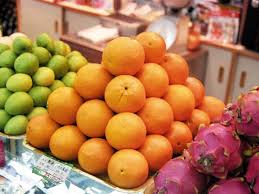
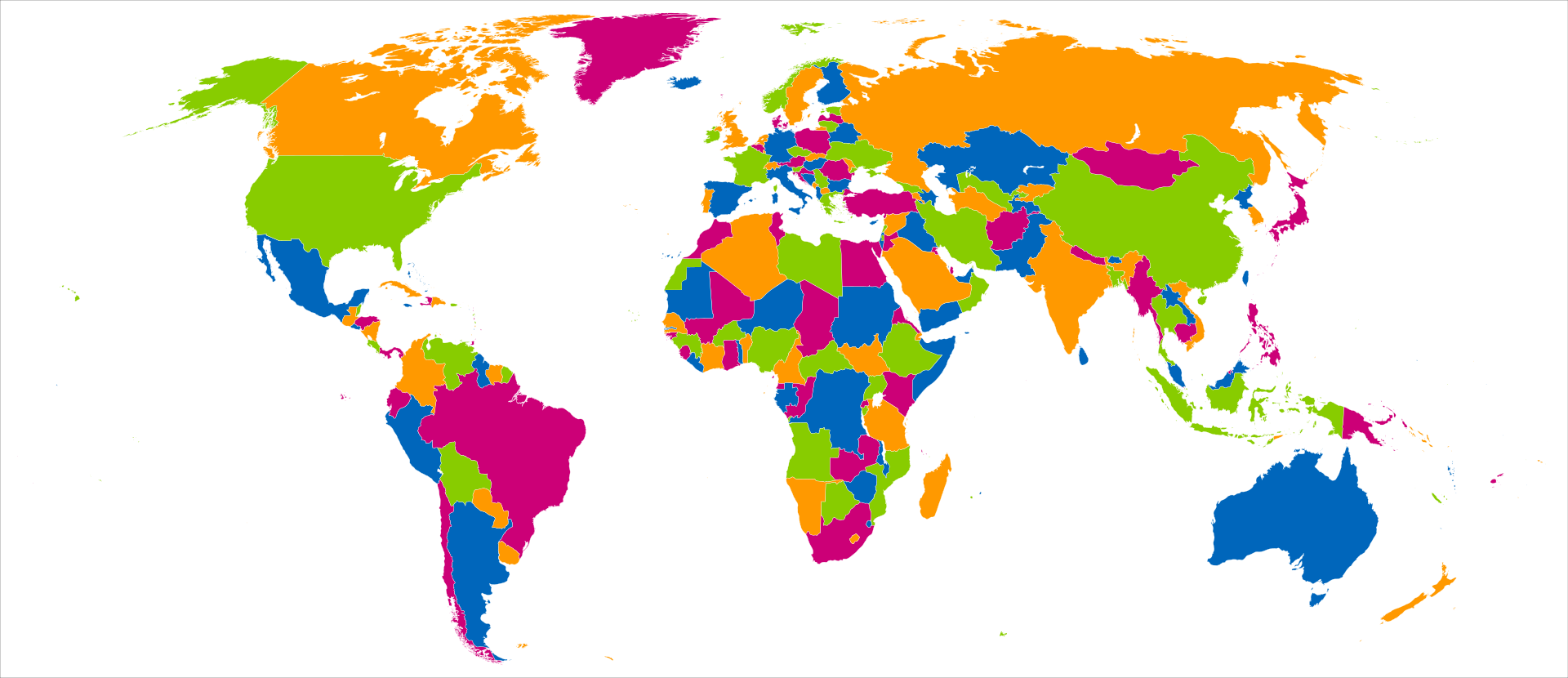
There are some difficult Theorems that seem conceptually obvious we were not able to prove without the help of interacive theorem proving. As far as I’m aware, the two most famous examples are Kepler’s Conjecture (the best way to stack oranges) and the Four Color Theorem (you can paint a map with only 4 colors so that no neighboring regions have the same color). They both seem kind-of obvious, right? Yet prior to the Flyspeck Project for Kepler’s Conjecture, all proof attempts had steps that didn’t convince other mathematicians (as rigorous enough).

Interactive theorem proving is also used for cool things like program verification and security.

Automatic Theorem Proving

Automated theorem proving systems aim to prove whole theorems for us. We give them the Conjecture and the Premises, and then it proves that, fx, \(ab = (-a)(-b)\) for us, without leaving out any steps. Actually, it’d be even better if we gave the ATP (automated theorem prover) the Conjecture and our full mathematical background theory, and it figured out what good premises would be. It figures out on its own what it needs to prove the Conjecture. After that if the ATP finds useful, interesting, or meaningful mathematical conjectures on its own, then we have a bonafide “AI mathematician”.

It has been done. Paul Erdős even proved an automatically generated conjecture!

ATP aims to be a self-sufficient general theorem prover, not just a proof assistant. Succeeding at developing an AI theorem prover may be sufficient for developing a General AI. (This, alas, means that ATP is really damn hard. Hmm.)

ATP and ITP are related.

> Large formal libraries of mathematics (which couldn’t be devleoped without ITP) are indispensible training data for ATPs.
> ATPs are general “gap-fillers”. If none of the ITP tactics can fill the gap in your proof, maybe an ATP can get it.

When ATPs are used to help ITPs they are called hammers.

My work, ProofWatch, is done at this intersection. We did some modifications to the ATP E and experiments with how to use it. This both makes E a stronger ATP and provides formal mathematicians with more intuitive ways to guide E (to E work with the particulars of the given Conjecture/problem and its related background theory).

E Prover

E works on First Order Logic (rather than Higher Order Logic which can express more but is less well-behaved).

E is a “refutational theorem prover”. This meeans that E does a proof by contradiction. This works because in line with the Law of Noncontradiction one cannot in logic have that both “Zar is a cat” and “Zar is not a cat” are true. Actually, one takes the Law of Excluded Middle that: Either Zar is or Zar is not a cat! There’s no Zar is neither a cat nor not a cat option. In some less-popular logical systems this option can be present.

So we know that \(\mathsf{Premises} \not \vdash \bot\) (which reads, “the Premises do not prove False (contradiction)” or “The Premises are axioms or true, consistent Theorems”).

Thus to prove our Conjecture we try to show that we can prove False (the Empty Set \({}\), actually. This is done by looking for a contradiction in putting the Premises and NOT the Conjecture together.

\[\mathsf{Premises} \wedge \mathsf{not Conjecture} \vdash \bot\]

\(\wedge\) means “and”. Because we know the Premises are cool, we know that the problem comes from the negated Conjecture. So the Conjecture must be true in the background theory of the Premises. Voila. We has a proof :).

What happens if the Conjecture is false? Then E will run for the lifetime of our Sun doing every possible inference (logical step) to try and prove False. If it finishes we still don’t know for sure that the negated Conjecture is true or that the Conjecture is false!

There’s this lovely hypothesis called the Continuum Hypothesis.
Take:
> The Integers, \(\mathbb{Z}\), numbers like -1, 0, 1, 2, 3, . . .. Countable numbers.
> The Reals, \(\mathbb{R}\), numbers including \(\pi\) and \(\frac{7}{22}\).

There are infinitely many Integers and there are infinitely many Reals.

The Reals are infinitely bigger than the Integers. They are so much bigger that the Integers are best considerd to have size “zero” in the context of the Reals.

The question: is there a type of numbers whose size is between Integers and Reals? \(\mathbb{Z} < \mathbb{?} < \mathbb{R}\).

The weird thing is that we can prove that we can’t answer this question according to the most common foundation of math (ZFC set theory). If there are such numbers, that’s ok with ZFC. No contradiction. And if there are no such numbers, that’s also ok with ZFC. No contradiction.

Philosophically, this can be quite interesting to ponder.

So waiting to see if E finds a contradiction or the Sun explodes first is a pretty bad idea: even if it fails, it may not tell us much.

In practice E is run for 5 to 60 seconds. Running E much longer usually doesn’t help much. Eventually E gets lost in that insane number of possible inferences and combinations of the Premises and negated Conjecture. On plus side, E can find proofs shorter than the ones Humans may find sometimes. This is somewhat fitting for E’s use as a Hammer in an ITP system where the human looks at the big picture and uses E to hammer away at smaller details in some steps of a proof.

Premise Selection

Stuff like the Continuum Hypothesis and getting lost in the deep, deep forest of math are why premise selection is so important.

If you include too many premises, E will get lost and have trouble.

If you include too few premises, E may be missing the secret ingredient to a proof.

Humans are pretty decent at premise selection.

We have used the k-Nearest Neighbors (k-NN) algorithm for premise selection in the past. Recently a fellow junior researcher worked on ATPBoost has used XGboost, a gradient boosted decision tree method, to improve premise selection.

In my research, I use a well-tested Premise selection and concern myself with other challenges.

E’s Heartbeat

E works on [clauses], stuff like the following, where \(\vee\) means “or” and \(\neg\) means “not”

1. \(aunt(zade)\)
2. \(sister(zade, zar) \vee \neg aunt(zade)\)
3. \(female(zade) \vee \neg aunt(zade)\)

The proof of \(a \times b) = (-a) \times (-b)\) at the start was very neat. If I were trying to figure out how to prove it from scratch (instead of cheating and looking it up; although I presented it differently than on the website where I found a proof), then my scratch sheet would be messy. I’d start doing some inferences, logical steps, that don’t go anywhere. They’re not wrong or illogical steps (ok, I’m not a computer, so maybe a few), but they don’t help in the proof.

> How do we know which Premises to use?
> How do we know what to start with? I started with equality (\(a = a\)) and one side of the Conjecture. But how did I know to do that?
> Once we choose a Premise to use, how do we know what to use it on?

The proof looks very neat and clean at the end, but there’s a lot of confusion on the way.

E takes a very simple approach (and there are many options/parameters you can tweak to change E’s strategy).
It’s a bit brute-force.

E keeps track of clause it’s processed, P, initially empty. And E keeps track of clauses it hasn’t processed, U, initially all the Premises and negated Conjecture.

Then E, by some heuristics or strategy, chooses a clause.

Let’s look at an example of how E processes clause 1 to 3 (even though there’s no Conjecture here). First we put them all in U.

Then E chooses #1 \(aunt(zade)\). Nothing special can be done, so E puts it in P.

Then E chooses #2. When E chooses a new clause, it doesn’t know what to use it on, so E uses the clause on EVERYTHING in P (can you guess why E gets lost if it runs for a long time now?). In this case we know that Zade is an aunt, so if “Zade is the sister of Zar or Zade is not an aunt”, then we know that Zade is the sister of Zar, \(sister(zade, zar)\). We have a new clause, and add \(sister(zade, zar)\) to U, because we haven’t done anything with it yet.

A simple strategy is FIFO (first in first out), so E takes #3 next. “Zade is female or Zade is not an aunt”. Looking at #1 and #3, we get a new clause: \(female(zade)\). Add it to U. #2 and #3 don’t tell us anything interesting (although one could hypothesize sister(zade,zar) and female(zade) are related).

Next E takes #4, “Zade is Zar’s sister”, and try combining it with 1-3, but it doesn’t tell us much. #5, “Zade is female”, also doesn’t tell us much.

Then U is empty. So E terminates before the Sun. Our logical inference engine E told us two new facts: Zade is female and Zade is Zar’s sister. These were implied by the Premises, but now we know them precisely :).

In practice, E can generate millions of clauses easily. And each time P grows, E generates even more each step. Many generated clauses are redundant (they in some way say the same thing, at least in the context of other clauses in P) and can be pruned. But this doesn’t help enough by itself.

This is called the “Given Clause Loop”. The given clause is the one chosen from U to put into P.

1. Choose “given clause”.
2. Do inference with “given clause” and all clauses in P.
3. Process generated clauses: simplify, remove redundant ones, move to U, etc.

When E chooses from among so many clauses in U, we need to help E choose intelligently!
This is what Stephan Schulz (the primary creator of E) said in his AITP Talk:

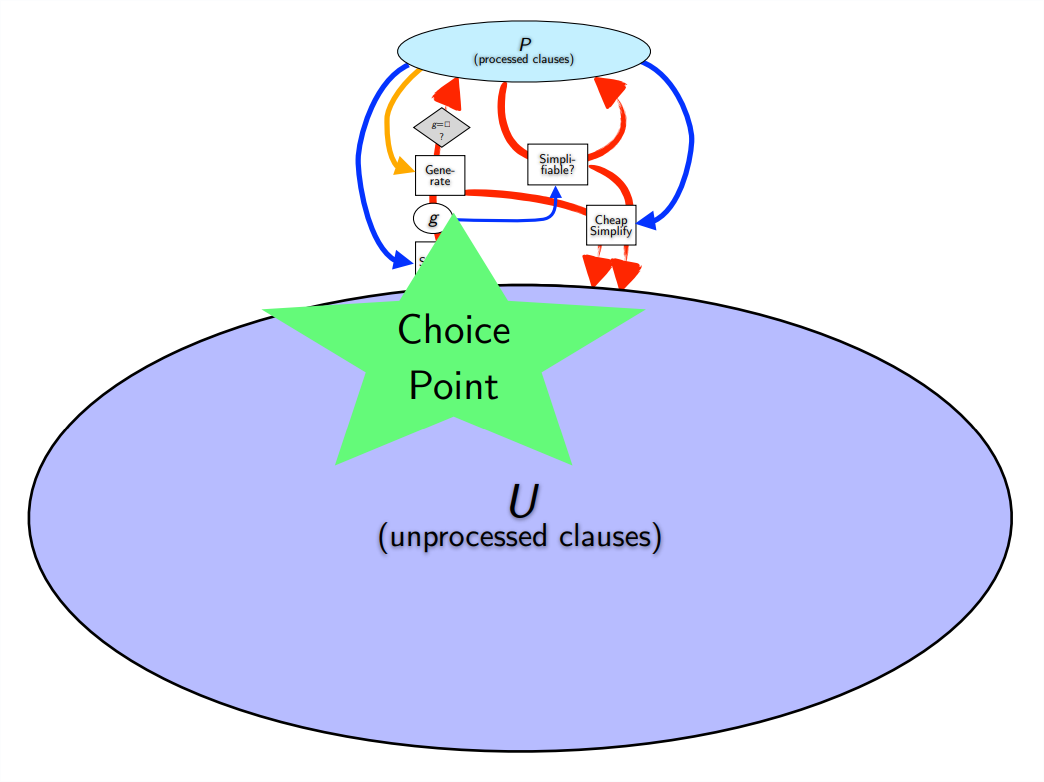
The Choice Point is choosing which clause to process next.

Why not steps #2 and #3?

I’m not entirely sure, to be honest. Humans definitely put a lot of care into them; however we may unconsciously do many inferences and discard them, at least in some approximate way.
E needs to be very fast because it searches through insane numbers of clauses. (If E were smarter, things may be different. However, there may be use for a fast ATP component anyway.) The already sophisticated heuristics may be good enough for processing general clauses (#3) that the potential gains from improving it without improving Given Clause Choice are lower.

Theoreticians like theorem provers, like E, to be “complete”. This means that if there is a proof of the Conjecture, E will find the conjecture.

So if we don’t do inference with the given/chosen clause and all the other clauses in P, then we have to keep track of which clauses we didn’t do inference with. And a strategy for choosing when to try these. This slows E down, and given E’s limitations, may also not help much. (There are some ways to limit the clauses in P one needs to do inference with and stay complete. Don’t worry. My predecessors haven’t been lazy.) Moreover the problem of figuring out which clauses in P to do inference with may be similar to the problem of choosing a given clause, but with fewer potential gains.

(It may be interesting to hear feedback from someone who knows better.)

Given Clause Choice

This choice point is what my research focuses on.

One of the cool things about E is that one configure a complicated strategy telling E how to choose clauses to look at next. There are smarter things than what I did in the example above: FIFO. E running after each clause in the order they were found is not that smart; although when I imagine E like a dog, it looks really adorable and cute.

It might be smarter to prefer small clauses. There are many reasons. There are weird traps in logic where one does inference with some clauses and they just keep getting bigger and bigger in a way that doesn’t add annnny interest. Imagine you’re looking for “23” but then you guess “77”, which encourages you to guess “78”, “79”, “80”, etc… and you keep getting bigger. So you can tell E to prefer smaller clauses. And there are many ways to weigh clauses, many ways to count the symbols.

And these methods can be combined: “Hey, E, sometimes do FIFO. But usually choose short clauses. Ok?”

Clauses like \(aunt(zade)\) are called “unit clauses” because they only make one claim (that is they have one predicate) instead of “This or That or The Other Thing” (three claims/predicates). Dealing with these can be very fast and useful – and even generate new unit clauses. That’s why E has something called PreferUnits that tells E to choose and process all unit clauses and then other ones.

Now we have two kinds of stragies: one assigns a number, like weight, and the other splits clauses into a different queues.

The ones that assign a score are called “weight functions” and the ones that queue clauses are called priority functions. To make things weirder, FIFO (first in first out) can be either of them! FIFO can make a separate queue for all clauses generated at the same time (that is, by the same given clause) or FIFO can score and order the separate queues (say, of unit clauses and then others).

E organizes this with “clause evaluation functions” (CEF). They combine weight and priority functions. To show the order, one writes:
\(CEF = \mathsf{weight\_function}(\mathsf{priority\_function})\)
\(CEF = \mathsf{FIFOweight}(\mathsf{PreferUnits})\)

. . . And a strategy is then a combination of different CEFs: do CEF1 20% of the time, CEF2 60% of the time, CEF3 5% of the time, and CEF4 15% of the time.

This is all very complicated (and weight functions can have many numeric parameters, for example: \(SymbolWeight(PreferUnits,0.99,0.99,1,20,0.99,\dots\)).

Who has time for this?

. . . Computers!

A colleague and my supervisor did work on automatically finding good strategies for E.

These are all good strategies, but we find some Conjectures can only be proven by some and not others. So it’s best to try an ensemble of them (such as 5 of them) and hope one works.

It’s possible these strategies still aren’t smart enough: running 32 different strategies for 5 seconds each they only get \(42.6\%\) of Mizar Mathematical Library, the set-theory based formal library of math we use.

One way to remedy this is by making a smart clause evaluation function.

The same colleague and my supervisor used machine learning methods to quickly determine whether a clause will be useful or not. They used an SVM (Support Vector Machine). The goal of an SVM is to take a bunch of Xs and Os on a piece of paper and draw a line between them. Xs and Os are different, so the SVM tries to find a line that is so good if one is given a new X to draw on the paper, it will also be on the right side of the line. This is called “classification”. The cool thing about SVMs is that they draw a line in an infinite-dimensional space (unlike a piece of paper, which is 2-dimensional), so the “line” an SVM draws can actually be very squiggly or a circle when you put it on the 2-dimensional piece of paper! Very cool, really. And they’re fast (unlike deep neural networks for now).

They made E prove many Conjectures and then labeled every clause used in the proof X and every clause not used O. Then they trained the SVM to classify clauses as “useful” or “not”, X or O. They then turn this into a clause evaluation function (and include a clause length weight as well, because short clauses are nice).

Now E can learn from stuff it did in the past. Maybe E can learn different SVM classifiers for different Conjectures, or at least for different kinds of math.

They called this system ENIGMA.

ProofWatch

This is where ProofWatch comes in. It’s another way of choosing the next given clause for E based on Conjectures E has already proven.

The high-level idea is similar to ENIGMA.

Recall that math is a dense, rugged forest (imagery courtesy of Godel, Escher, Bach:

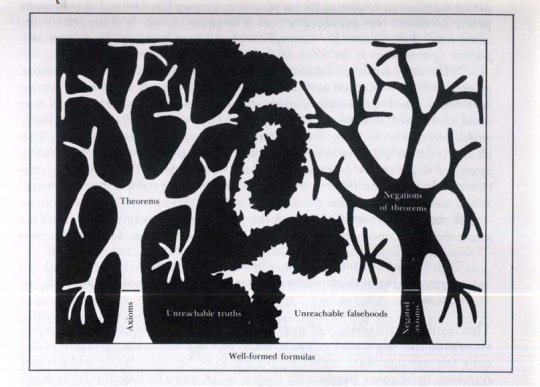
And the way through these ‘trees’ of Theorems and Negations of Theorems is riddled with weird, twisted logical pathways, hallways and vines that somehow curl through themselves infinite times:

Each proof of E’s we have is a path through this wild forest.

ENIGMA tries to learn to recognize a path in the forest: sometimes they’re not as clear as wide dirt roads through the park.

If a clause is on the “useful” side of the SVM’s ‘line’ then it “looks like a path”, it looks like a clause that is part of a proof.

You might wonder: is it ok that ENIGMA just learns to recognize if a clause is part of A PATH rather than THE PATH FOR OUR CONJECTURE?

It’s almost ok.

A cool thing about proofs by contradiction is that “all paths lead to the same place”: emptiness.

And classifiers can be trained for specific fields of math.

However, yes, even if a clause on is a path, that path may require a Premise or negated Conjecture clause that we don’t have in our current mission. It’s like exploring a dungeon in a video game: you played the game as a small character already, and now playing as a big character you try to follow a similar path but then run into a door you can’t get through. Drat. Even though it IS a path, you can’t walk it with this character. We do something to help remedy this later.

There are 30 characters, and you have walkthroughs for 20 of them in this game. ENIGMA looks and the walkthroughs and what the author did while playing the game to make the walkthroughs and tries to learn to recognize the “right sort of thing to do”.

ProofWatch just looks at the walkthroughs (proofs of other, related Conjectures). ProofWatch takes the walkthroughs along with it as it tries to beat the game with a new character (a new Conjecture). Every step (new clause) it sees if this step leads to something in a walkthrough it had before (a clause in another proof). If this step (clause) leads to part of another character’s path (Conjecture’s proof), then it’s a good bet. Maybe it’s part of this character’s proof. So ProofWatch then gives the clause better priority in E.

Another question: if we start following the path of a clause that matches another proof, should we try to keep following that path?

We decided YES. So children clauses (ones generated by the given clause) of one that matches another proof get some boosted priority too. And just in case this isn’t actually a good path for this new character, after a few generations of children, ProofWach doesn’t give good priority anymore.

Another question: we generate different clauses that lead to three different proofs. Three paths to choose from. Three other characters walked a route like this in the game. How do we choose which to follow first?

In ProofWatch, we keep track of how often our exploration has intersected other proofs. The more similar, such as the path in a game for another big character (as ours is big), the more relevant that proof (probably). So we make the priority boost depend on the relevance, on the intersection.

It would be good to make the priority boost depend on how close the clause in the other proof is to the end of the proof/game. All proofs lead to the empty set \({}\). The closer the better. However, we have not implemented this yet.

That’s the high-level picture of what E does with ProofWatch.

It’s similar to ENIGMA in how it helps E at the choice point with given clause selection, but ProofWatch literally looks at the clauses in other proofs instead of learning a ‘linear’ model to judge clauses by.

Below I’ll discuss some slightly more technical details and then talk about how it did.

More Formal Details

E has this feature called the watchlist, since 2004 at least. The watchlist is a list of clauses that E compares generated clauses to, and if there’s a match, E boosts the clause priority. E does this with a priority function: PreferWatchlist (like PreferUnits in the example earlier).

For whatever reason, no one had successfully used E’s watchlist feature on some benchmarks, even though it was around for over a decade.

Another ATP is Prover9, which has a good Wikipedia page. It includes an example of the traditional “Socrates is mortal” proof.

Prover9 has a feature analogous to E’s watchlist: the hint list.

I actually like this terminology more. It sounds cool to be giving the theorem prover some hints.

Prover9’s hint least feature was used to prove a difficult Conjecture in loop theory in many types of loops, and they’re still working on the main AIM Conjecture. The main researcher helps choose hints by hand though! He also tries various frequency counting heuristics, distance to the end of a proof (ahead of us in many ways), etc. So even though he works directly with an automated theorem prover, he’s doing interactive theorem proving.

Now, how does E see if a generated clause C leads to a watchlist clause W? Recall before we had this \(\vdash\) symbol? (\(\mathsf{Premises} \wedge \mathsf{not Conjecture} \vdash \bot\)). \(\vdash\) means that we can get from the Premises and negated Conjecture to \(\bot\), False, emptiness, via following some path of logical steps.

So it’d be cool to do the same. If \(C \vdash W\), then we can get to clause W from clause C via logical steps. W led to \(\bot\) before. So maybe E should make C the given clause and see where C takes it. (Why don’t we just go directly to W? W may have parts specific to the proof/path W is in that don’t help for the current Conjecture.

Unfortunately. Logical entailment/consequence, more or less this \(C \vdash W\) thing, is undecidable in general. In general it’s impossible to tell if \(C \vdash W\) or not. Ouch. Logic is a deep, dark, and scary forest, isn’t it?

Computer Science is too. The deceptively simple Halting Problem is undecidable. There is no method to tell, in general, if a program with some input will stop or run forever. A lot of the time we can, but in general, nope.

Fortunately for us, there’s something called \(\theta\)-subsumption that’s a good approximation to logical entailment. \(C \vdash W\) means “when C is true, W is true”. When \(aunt(zade)\) is true \(aunt(zade) \vee uncle(zade)\) is true. If Zade is an aunt, then Zade is an aunt or an uncle (and maybe she’s both!). Clauses are a bunch of predicates/statements connected by “or”. The way “or” (\(\vee\)) works is that if one predicate is true, then the clause is true. (This is like checking if \(C \{aunt(zade)\}\) is a [subset])https://en.wikipedia.org/wiki/Subset) of \(C \{aunt(zade), uncle(zade)\}\).)

We write \(C \sqsubseteq W\) for C subsumes W. And if it does, then \(C \vdash W\). So there are some cases where \(C \vdash W\), but C doesn’t subsume W. Such cases are with self-recursive clauses: clauses that include themselves . . .. Subsumption is an NP-Complete problem (one that can’t, in general, be solved goodly fast relative to the size of the problem), but at least it is solveable!

However, subsumption only gets interesting when we have variables. Variables are for when we have a rule that holds for anyone, not just \(zade\):

1. \(aunt(zade)\)
2. \(female(X) \vee \neg aunt(X)\)
   (which can be read “If X is an aunt, then X is female”)

Just as before, E can conclude that \(female(zade)\) is true by setting \(X = zade\). This is called a variable substitution. Plugging in “zade” to “X”.

It’s what you did when solving equations \(x^2 = -1\), so \(x = ?\). You figure out what number to plug in to “x” so that the equation is true. And in cases like \((x-1)^2 = x^2 + 1^2\), the equation is true no matter what “x” is. It’s just useful if we need to change the form we’re working with or get some specific result. #2 is true like this, but maybe learning \(female(zade)\) will help with proving our Conjecture.

Proper \(\theta\)-subsumption asks if there is some variable substitution/setting that makes clause C be contained in clause W. This is a bit like saying C can be more general than W. If we know that Socrates is mortal, we don’t necessarily know that all men are mortal. But if we know that all men are mortal, then we also know that Socrates is: we can substitute \(Man = socrates\). Some examples:

1. \(human\_rights(X) \sqsubseteq human\_rights(zade)\) (with \(X = zade\))
2. \(female(X) \vee \neg aunt(X) \sqsubseteq female(zade) \vee \neg aunt(zade)\)
3. \(sister(zade, X) \sqsubseteq sister(zade, zar)\) (with \(X = zar\))
4. \(sister(sally, X) \not \sqsubseteq sister(zade, zar) \)
5. \(sister(zade, X) \not \sqsubseteq sister(Y, zar)\)
6. \(sister(zade, X) \sqsubseteq sister(Y, X) \vee \neg aunt(Y)\) (with \(Y = zade\))
7. \(\neg aunt(zar) \sqsubseteq sister(Y, X) \vee \neg aunt(Y)\) (with \(Y = zar\))

Notice some weird things? It’s a bit strange. #1 makes sense logically, and some sense if “X” is restricted to humans. But what if “X” can be anything, dogs or 3? #2 is better. #2 is a nice general rule that implies a zade-specific rule. #3 is weird too: if everyone is Zade’s sister, then Zar is. These cases are weird for two reasons. First, general knowledge with variables will usually be in forms more like #2; single statements are likely to just have actual particular people or numbers inside (called ground terms). Second, in logic the scope of variables is often included. #2 may be true only for “X” that are people (not numbers). Or we may say that “there is an aunt”, and then we can set “X” equal to that aunt.

In #4 we see that different particulars mean subsumption can’t happen.
in #5 we see a case where both sides can be solved (unified), but subsumption can’t happen because we can only find variables on one side.
In #6 we see that we don’t have to substitute something for every variable, just enough for equality with one term of the right-hand clause.
In #7 we see that the substituted-equality can be with either predicate.

So it’s a bit weird, but in practice clauses don’t get that big and it works pretty fast.

#2 is a good example of why when ProofWatch finds a clause \(C \sqsubseteq W\) for W on a watchlist from another proof, ProofWatch chooses \(C\) and doesn’t take \(W\). Clause \(C\) may be more general. And perhaps \(zade\) was something particular to W’s proof, and not relevant in the present proof. We have a different character now. Also, because C only has to be made to match ONE predicate in W, a short clause C could match a long clause W. We’d be taking in a lot of extra baggage to try and actually use W.

That’s why ProofWatch just uses other proofs to tell which clauses are good directions to look for a path/proof in.

Watchlist Strategies

We tried some ways to vary or add the watchlist checking priority function PreferWatchlist into the strategies we previously automagically found.

To cut a long story short, the best thing we found (especially for ensemble/combined success/coverage) is to just replace ALL priority functions in the strategies with PreferWatchlist.

Boring. Simple. Works.

(And a surprise finding was that replacing all priority functions with ConstPrio, a priority function that does nothing, also improved the strategies a bit. With our strategies, it seems weight functions do the job well – better – without help from too-crude priority functions!)

Watchlist Creation

To be honest, the watchlist for E and ProofWatch doesn’t actually have to be “steps from other proofs”. You can put anything you want on there! The logic is the same “these are smart things to do in the game, so if we find a way there, follow that way.” If you know of some pretty good signs in the forest for finding emptiness (\(\bot\)), then those could also go on the watchlist.

We did a few tests of choosing the most frequent/common proof clauses to put on the watchlist. So now they don’t come from any proof in particular. No proof-completion or relevance counting. The tests indicated that this can help. (Ok, we probably should have tested this more thoroughly.)

The Mizar Mathematical Library has a bit over 1000 articles. An article is a collection of Theorems (Conjectures with proofs) on specific topics. There are articles on Integers, Reals, Boolean Algebra, Integrals, Complex Numbers, Turing Machines, etc. You can browse the list, and even the Theorems and Proofs in a nice htmlized format.

One can’t just take all proofs E has ever done and put them on the watchlist. This would be awesome, but E can’t do that fast enough. Checkeing \(C \subseteq W\) isn’t that slow, but so far above \(5,000\) clauses \(W\) on watchlists, things start to slow down. If there were some smart and fast way to only check some of the possible cases, that’d be great.

The simple and easy option that works is to group proofs by Mizar article. If we have a Conjecture on Integers, then only include proofs about Integers. (A bit like only looking at walkthroughs from other big characters that use swords.)

We also used k-Nearest Neighbors (k-NN) to select “near” or “similar” clauses or proofs to the current Conjecture. (Details on how we put Conjectures into a form so that we can see which are closer can be found in the ENIGMA paper. The basic idea is to treat logical formulas as trees, assign a number to symbols, operations (like \(+\)), etc. Then we take things like subwords for trees. For example, the subwords of length 3 of “word” are “<wo”, “wor”, “ord”, and “rd>”, where < and > are for start/end of the word. We add up the formula-tree-subwords and put them into a vector form: \((0,0,0,0,0,0,1,0,0,13,0,0,\dots)\).

We even helped ProofWatch learn! We had E do a bunch of proofs using k-NN advised watchlists, and then kept track of which proofs in the watchlists were actually useful and which were not. Then we fed this data, “om nom nom”, into k-NN as well.

The k-NN watchlists are better than the Mizar article-based watchlists. (Which kinda indicates k-NN can also be improved upon.)

Experimental Plots

We did a bunch of experiments with 5 of the 32 E strategies we have. These 5 are good ones. They prove \(80\%\) of the Conjectures proven by all 32 combined.

The only frequency test you’ll see. We take the top 10, 100, 256… clauses found in E proofs and throw them on the watchlist. Get them fresh! Get them hot!

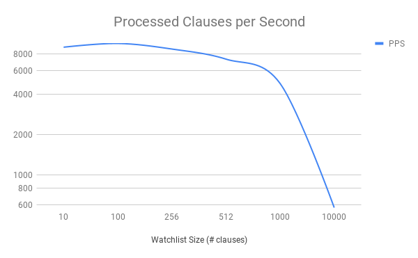
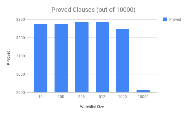
Analysis: ouch! OUCH!

E’s speed goes down fast with the size past 1000. As long as the watchlist size is not over the cliff, the results look about the same.

(Caveat: this is only one strategy with Mizar article watchlists.)

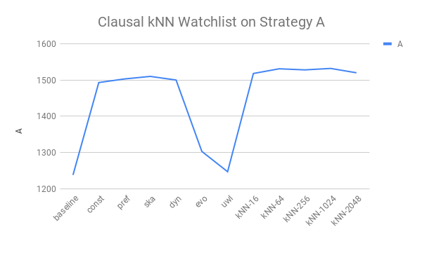
Next is the big one: we test some ways of using ProofWatch on our old “baseline” strategies (along with the “const” no priority function option). We sample 5000 out of 57897 Mizar problems. And believe it or not, we discussed some different ways of using the watchlist feature in E. The pref option just uses the PreferWatchlist priority function and considers the watchlist one big list of clauses. We discussed keeping track of which proofs each clause comes from to pay more attention to proofs we see a lot, right? This is called dyn (for dynamic). The one called evo is a default E prover strategy for watchlist use! (Which is a bit unfair as then there’s not as much variety when combined with our 5 strategies.) The uwl one is surprisingly bad. It combines the priority functions in the baseline strategies with PreferWatchlist. Maybe it’s bad for the same reason const is good. Finally ska is needed for annoying technical reasons. When there’s a clause such as \(\exists X. aunt(X)\) we do something called skolemization: since there is someone who is an aunt, let’s just call her \(skolem\_gal\) and write \(aunt(skolem\_gal)\). Often this works. But recall that you can’t substitute anything but a variable, so now if the skolemization is inconsistent, we can’t do subsumption properly. ska is a version of pref where we treat all skolems the same (even though this can sometimes be wrong and mislead us).

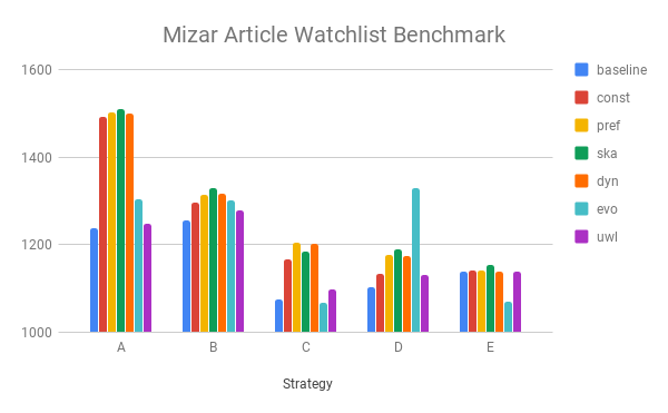
Analysis: Hey, funny, evo does really well in combination with strategy D for some odd reason!

Analysis: A and B are killer. Yet the 3 others add a good 500+ to the total number ;-).

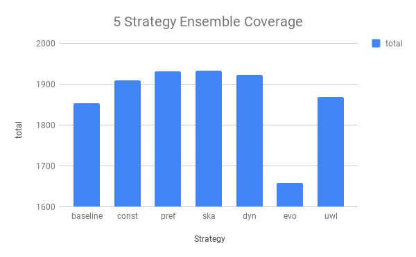
Analysis: Weird, on E ProofWatch doesn’t do much.

Analysis: ska for the win. The similar pref and dyn are about the same, too. const is not far behind, whoa.

Comment: It’s a bit surprising the smarter-trick dyn doesn’t do better. Is it because of the watchlist-creation method?

Comment: So far, so good. Taking walkthroughs with you helps. Using prior E proofs helps E prove more. Yay ProofWatch.

Ok, another case where there is insufficient testing. But we did a bit! We used kNN to suggest watchlists for our 5000 test Conjectures. It suggests each clause on its own merit (so we can’t use dyn, as it dynamically boosts priority relative to how much of each proof we’ve seen). We did this only with proofs from strategy A, so we can’t examine its ensemble performance. The verdict: k-NN does better. Not a damn lot, but a goodly amount. Watchlist size doesn’t matter much: we didn’t hit the cliff.

Next are the results for using kNN to suggest whole proofs to put on watchlists. Will dyn shine?

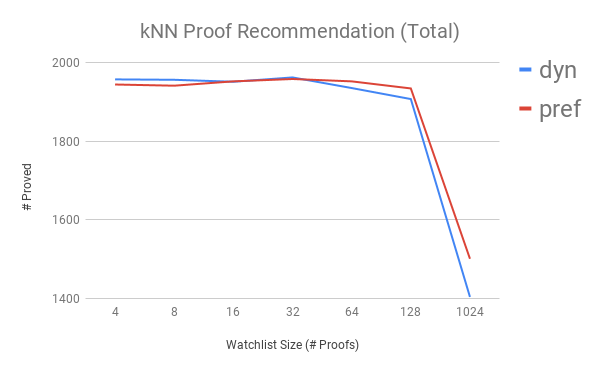
Analysis: Performance slowly rises to 32 proofs (about 1200 clauses), and then they droooooop.

Analysis: dyn shines, a bit, but slows down faster and harder.

Analysis: pref does better with kNN proof recommendation than kNN clause recommendation. Bit surprising.

Comment: The following comparison for ecah of the 5 strategies is interesting.
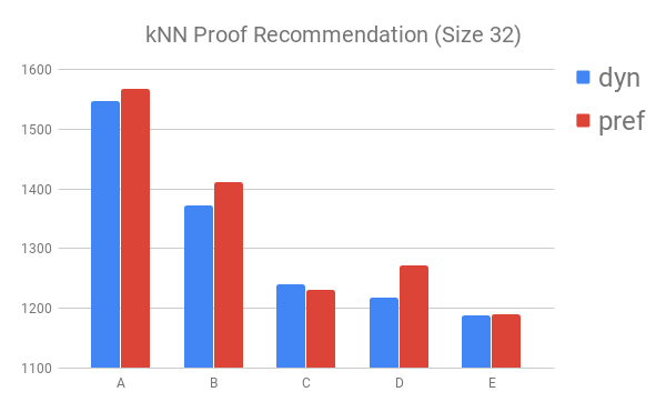
dyn has a slightly better ensemble coverage of proofs than pref, even though it does significantly worse on all strategies but C.

This is an interesting and important point about why ensemble coverage matters more than doing well with just one strategy (especially as running strategies over 60 seconds doesn’t help much).

I find it curious how a strategy we thought would guide E better, dyn, seems to guide E better in diverse Conjectures, but in each individual run of E miss out on more proofs. Is this because it is slightly slower? Or because the way we measure proof relevance to the current Conjecture dynamically isn’t that good yet? Hmm . . ..

Anyhow, next is kNN Round Two. We take a greedy cover of our results on the 5000 test-set to find the 5 new strategies that cover the most; run these on the full 57897 Conjectures; and add to knn the data on which proofs on the watchlists were actually matched (subsumed) and used in a proof. 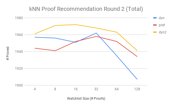Lo and behold, dyn2 learned and does better.

The peak is now at 16 proofs, meaning the recommendations are really getting better. Coolio.

There’s one other smart thing to try I mentioned earlier. Once we choose a given clause based on matching a watchlist proof, it seems smart to give the clauses we generate with that given clause some extra priority too. A bit like inertia: once you take a step down a path, why stop immediately? We’d keep walking a bit before trying another path. This is called dyndec2 for dynamic with decaying priority (each generation). 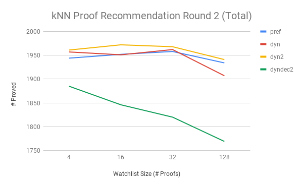Whoa there! What gives?

This was supposed to be smarter yet it’s worse and its performance certainly decays faster with watchlist size!

Ok, this is understandable. The way a priority queue works is that if Clause C1 has priority \(40\) and C2 has priority \(39.99999999\), then (as lower priority is better) C2 will be chosen before C1. So if \(C \sqsubseteq W\), C matches a watchlist, then all of C’s children will be chosen before any clause that doesn’t. This means that with this dyndec2 strategy, the watchlist has to be very intelligently focused: otherwise ProofWatch may be led into weird places or distracted from the way.

At this point I got curious.

What one wants most is ensemble coverage. We want to be able to prove some Conjectures that E can’t without using the watchlist. So totals are cool, but what about how many proofs we get that aren’t covered already?

To figure this out, I took top-5-greedy-covers for the primary methods in our study and compared them to baseline and const to see how many new boiz we got.

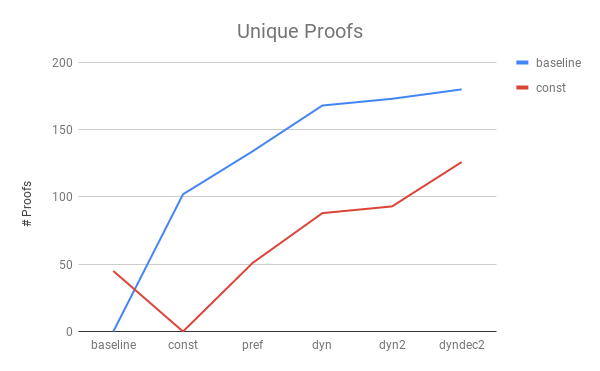
Pretty cool. dyndec2 helps E find a bunch of proofs that the other methods didn’t, even though its solo performance doesn’t get such high numbers. Fortunately, strategies can be scheduled to work together and complement each other.

Comment: The baseline methods get around 45 proofs const, pref, dyn, and dyn2 don’t, but 135 that dyndec2 doesn’t. So it really just diverges a lot!

Unsurprisingly then the best ensemble of 5 strategies in our experiment contains 3 dyn2s and 2 dynden2s. Does \(7\%\) better than we were doing before.

There’s definitely lots of room for finetuning this technology.

In addition, ProofWatch can output a vector telling a user (such as a Interactive Theorem Proving mathematician or AI) which proofs intersected the current proof-search most and how much. This is a bit like pieces of a puzzle that can be patched together to map out some of the mathematical-forest-territory. It should help one figure out how to target E at a specific Conjecture or Lemma (sub-goal) and hammer, hammer, hammer away.

Brief Example

Below is a brief example from the paper. Article Yellow 5, Theorem 36. You can click through the HTML Mizar if you want to really get it. Otherwise, the below is primarily to demonstrate the basic idea.

This is De Morgan’s Laws for Boolean Lattices (Boolean algebra with its “and”, “or”, “not”, “0”, and “1”)

theorem Th36 : :: YELLOW_5 :36
for L being non empty Boolean RelStr for a , b being Element of L
    holds ( ’not ’ (a "∨" b) = (’ not ’ a) "∧" (’ not ’ b)
          & ’not ’ (a "∧" b) = (’not ’ a) "∨" (’ not ’ b) )

This example is nice because it’s visually easy to see (and many people know De Morgan’s laws). The proof we get consists of \(27.5\%\) clauses guided by the watchlist and the proof gotten without the watchlist took E \(25.5\%\) longer. Exactly what we want to see: learning helping the ATP get to the end faster ;).

A Conjecture whose proof is heavily used in finding the proof for Yellow 5, Theorem 36 is Waybel 1, Theorem 85. It looks visually similar, but is done on Heyting Algebra instead. Heytting algebra is actually a weaker setting than Boolean algebra.

theorem :: WAYBEL_1 :85
for H being non empty lower - bounded RelStr st H is Heyting holds
for a , b being Element of H holds ’not ’ (a "∧" b) >= (’not ’ a) "∨" (’ not ’ b)

The ‘contextul’ proof vector we get at the end here is: 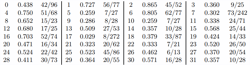Waybel 1, Theorem 85 is #6.

We can clearly see that a handful of proofs get matched significantly and others not that much.

One avenue for future research is to work on patching these fragment of the math-forest territory together.

Conclusion

That’s it folks.

I hope you learned something interesting.

I’m both surprised that there’s basic stuff like this that hasn’t been done much yet, and glad to be the one to get to do it :).

There are many avenues for improvement.

Stay tuned for musings on the relation of ATP, ProofWatch, and AGI.