Continuing the trend from the ProofWatch post, I’ll discuss some research casually (and perhaps less laypersony than before).
The short workshop paper (semi-published) can be found with Kalpa Publications: ProofWatch Meets ENIGMA: First Experiments. The conference LPAR is a cool one that aims to go “where no reasonable conference has gone before”, which brought it to Hawassa, Ethiopia :). Which, while cool, had the unexpected (but well-known) result of one-week eating the worst Ethiopian food I’ve ever had. Go figure, resorts are known for crap food. Witnessing the local culture and willingness to offer breast-feeding to young babies is pretty cool. And it was a good opportunity to visit iCog Labs (and, err, General Zod).
Anyhoo, the story continues precisely where ProofWatch ends (so go review if the brief overview is insufficient 😛).
Embodied Theorem Prover
The theorem prover E starts with its Axioms and (negated) Conjecture and wants to find a contradiction (reductio ad absurdum).
E works with about 20 inference rules, stuff like modus ponens (\(P \implies Q, P \vdash Q\) – “If P implies Q and P is true, then Q is true”).
If the Conjecture is true given the Axioms, the rules should eventually find a contradiction.
So E uses various heuristics to choose Unprocessed clauses (U) one at a time to do inference with (only pairing this chosen clause g with Processed clauses (P).
There are many nice heuristics to simplify clauses, remove redundant clauses, etc.
Nonetheless, P blows up, and you want good strategies for choosing the given clause g at each step to quickly find your contradiction, your proof.
(I wonder why no-one in the community seems interested in learning which clauses in P to do inference with. Maybe it’s obviously less important? It seems a bit like breadth-first expansion.)
Parameter tuning techniques for finding good (teams of) strategies help (see my colleague’s BliStrTune), but these still aren’t very smart. The information they have about the context of the proof-search so far is rather limited. And the strategies aren’t dynamic: you have one strategy for the whole proof-search run.
Someone does appear to be working on this: Dynamic Strategy Priority: Empower the Strong and Abandon the Weak. Apparently he makes Vampire (the evil non-free brother of E) record 376 features of the proof-search state (or context) and feeds these into a simple neural network to learn to dynamically choose which strategies to prefer.
This is a bit like deciding on your strategy for going through a maze or adventure course beforehand, and not adapting to what you see around you as you explore!
Kinda insane, right?
When I walk through a tunnel in the dark, I generally employ a strategy such as “keep my right hand on the wall and step cautiously”. Actually, for a simply-connected maze (without islands, bridges, etc) the “wall follower” strategy works: you don’t need to know much about “where you are in the maze” to get to the exit. You don’t need to create some mental model of the maze topography, situate yourself in the maze, speculate the sorts of paths, etc.
This brings up a good question: how many math problems can be solved simply by finding the “right strategy” to follow for the whole proof search?
Are there some problems not solvable via E’s inference calculus and strategy-parts?
(Answer: no because it’s refutation complete and a strategy that does First-In-First-Out one every 10,000 given-clauses will eventually try everything and find the contraduction (assuming there is one). Like the “wall follower” strategy, though, this strategy could take a very long time. Some strategy that uses more advanced reasoning and awareness of the particulars of the maze may find the exit much faster than the “wall follower” strategy. The same for E’s theorem proving: if we want to solve problems and prove conjectures in any reasonable amount of time, then yes there may well be such problems . . ..)
Another interesting topic (of marginal relevance to EnigmaWatch) is what does embodiment mean for a theorem prover?
What sort of world is the theorem prover exploring?
We generally think of embodiment as pertaining to our 3D+1 world: a biological animal or robot has a body enworlded. This body has some sensory interfaces with the world (skin, nose, ears, eyes, tongue, etc). And through these senses the embodied intelligence models its body and its world. These models situate and define the nature of problems emboddied agents face. Even better, the body+world practically motivate many solutions and attack paths!
Along with our embodied sensory interfaces are sense-making pathways that, in the case of vision, progressively detect more and more nuanced patterns in the ‘raw visual data’. Our high-level conscious intelligence gets to deal with a visual world where objects, edges, etc are already clearly dileneated.
Isn’t it lovely we don’t have to learn to identify objects from background over and over again?
If one has read Flatland: A Romance of Many Dimensions (which I reviewed as intellectually interesting but boring), then one has a glimpse at what it may be like to be embodied in a 2-D world. It’s actually a lot like a maze (where you don’t cheat and go OUT from the top 😛). Intuitions about navigation and construction will be quite different: 3 dimensions allow many interesting round-about methods (– actually more direct) that 2 dimensions don’t. And what might 4 or 11 dimensions allow?
So what sort of world is the theorem prover enworlded in, embodied in?
A logical one made up of clauses containng terms, variables and or (such as \(female(zade) \vee male(zade)\)).
Our theorem prover E sees a lot of these. A damn lot. Many mathematical terms defined in terms of others.
The clauses have relations to each other, so E knows which clauses gave birth to which others.
E’s heuristics are a bit like the first steps of pre-processing in the visual cortex, but E doesn’t have the full pipeline (which has backchannels too). 😢
Poor E.
How does E sense this logical lattice? E explores the clause-space from P via some new clause g, generating a bunch of new clauses its attracted to or repelled from (or just throws out). So far E doesn’t have much memory, and just instinctively (based on hard-coded heuristics) judges the new generated clause. A bit like a logical amoeba.
Memory and Learning 合体
This is where ProofWatch came in. Once our logical amoeba E solves some problems, load those proofs (a directed-acyclic-graph of clauses – or just a list) into E as a form of memory. Now when the amoeba looks around it seems some nice sugar and decides to follow that trail – err, E sees that a clause it generated subsumes (‘implies’) something it did before. Wheee ~ ~ ~.
Memory is cool. But there’s not much learning yet.
Recall ENIGMA (Efficient Learning-based Inference Guiding Machine) from the introduction of ProofWatch, done by a colleague.
It’s a simple learning system inside E (and while complex systems are cool, they’re too slow for this low-level part of the intelligence hierarchy 😜).
Like ProofWatch, ENIGMA learns from given clauses in its successful proof-runs (where it proves the Conjecture, solves the problem).
But ENIGMA uses ALL of them, not just the ones in the proof.
For example, below are some clauses from the proof (\(1\)s) that \((a \times b) = (-a) \times (-b)\) and some that are not in the proof (\(0\)s):
1 - \(ab = ab + (-a)(b + (-b))\)
0 - \(ab = ab + 0 + 0 + 0 + 0 + 0 + 0 + 0\)
1 - \(ab = ab + (-a)b + (-a)(-b)\)
0 - \(ab = a(b + 0)\)
1 - \(ab = (a + (-a)b + (-a)(-b)\)
These clauses are then fed into LIBLINEAR, a fast linear regression library, or into XGBoost (which learns a bunch of decision trees).
These machine learning software find models that tell E whether a clause is “probably good” or not.
To feed clauses into a machine learning library, one needs to somehow transform the logical symbols into a bunch of numbers (a vector).
For example formula \(f(x,y) = g(sko_1, sko_2(x))\) is represented as a tree:
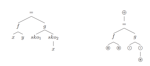
(Thanks for the image, courtesy of the article.)
Then from the tree perspective each “triple”, like (=,f,g) and (f, *, *), is considered a feature.
These features are numbered: 0, 1, 2, … |number of features| and then clauses can be mapped into this feature vector space 😉.
It turns out it’s good to add some more features (which you can see mentioned in a more recent ENIGMA paper).
One nice improvement is taking features for the Conjecture \(F_C\) and for the generated clause \(F_g\) and appending them together into a big vector of size 2 * |number of features|!
This revolutionary improvement allows E to learn to judge clauses, to explore its environment, relative to the problem it’s actually solving.
Now E can take into account the impression of the maze :).
– Alas, the Conjecture features don’t change for the whole proof-search.
This is where ProofWatch comes in :).
As we saw at the end of ProofWatch, E can count how many times generated clauses match each proof in its memory:
So now E has some sense about where it’s situated in the logic-maze: hmm, I’ve seen a lot of stuff from proof #1, #2, #6. Lots from proof #7 too (but only \(\frac{1}{3}\) of them).
This information should be able to help E determine which clauses to process next.
While this is cool, it’s also somewhat subtle: what does matching some of this other proof mean?
I can foresee some problems:
- Maybe a crucial axiom for proving #1 is missing when proving C, making confluence potentially misleading.
- Ok, the axioms are the same but the Theorem statement for #1 is actually kinda different from C. Maybe the high confluence means E is in the wrong part of logic-land.
- …
I like to think of the proofs in this context as sensor-probes.
Rods in eyes respond to different light frequencies (colors): and these proofs and their clauses are little detectors our logic-amoeba thrusts out into the wide unknown world. They react only to specific types of clauses.
So maybe there are better and worse types of sensors (not just proofs). Some combinations of proofs will be more telling than others. Maybe some proofs will be distracting (and overlap too much with others).
Anyway, these proof-matched-counts (actually the completion ratios) are a proof-vector that can be fed into the ENIGMA machine learner. Now E is authentically context-sensitive.
(Specifically, the proof-vector at the time a given clause g is chosen is stored, output, and used as the training data.)
MPTP Challenge
Because ProofWatch is slow (and ENIGMA wasn’t yet modded to work with large, sparse feature vectors), we chose a very small dataset to play with.
(Actually, the 150ish proofs that go onto the watchlist here is already pushing-the-limits speed-wise.)
Way back over a decade ago a famous theorem, the Bolzano-Weierstrass theorem (“states that each bounded sequence in \(R^n\) has a convergent subsequence.”), was used as a competition for theorem provers.
There are 252 theorems (problems) leading up to the theorem in Mizar. The question is how many of the problems can the ATPs solve (given the same axioms/prior-theorems humans used).
The organizer is good at cute graphics for his competitions (such as CASC, “The World Championship for Automated Theorem Proving”), so you can see the results. (By the way, the Large Theory Batch branch of the competition is the most interesting and tries to allow systems to learn on problems as they go.)
\(82\%\) proved ain’t bad, tho the best solo performance was \(75\%\).
The problems get progressively harder though.
A quick test with Vampire 4.0 resulted in \(87\%\).
We’ve come a long way in 10 years.
Results
(lool, aside: it’s much more fun presenting results when not feeling the need to compactify or sell them :’D)
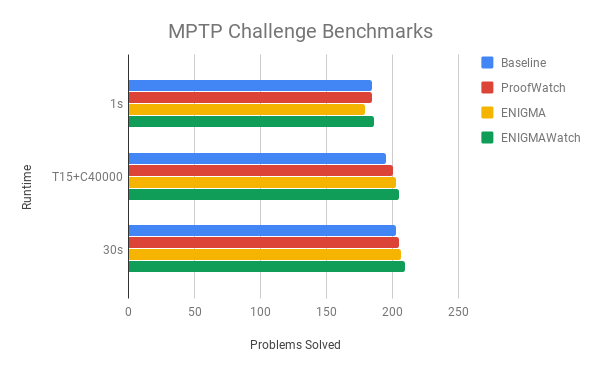
Okay, the results.
- Baseline, as in ProofWatch are 10 baseline strategies with proven theorems lumped together.
- ProofWatch is just a static watchlist (but it didn’t matter that much on this dataset, difference of like +/- 1 problem).
- ENIGMA does its learning magic from the results of Baseline (ENIGMA+strategy 01 learning from strategy 01’s proofs, etc).
- ENIGMAWatch does its learning magic on the output of ProofWatch, or slighly better, on the output of Baseline strategies run again and matching their watchlists (but not using them).
1 second per problem (per strategy) makes sense.
As does 30 seconds (which in sum means 300 seconds per problem, the time limits for the original competition). So E prover beats the old competitors solidly, but even fancy-shmancy ENIGMAWatch doesn’t beat vanilla Vampire. Yargh!
And \(T15+C40000\) means we count processed clauses, how many given-clause-loops, the prover gets to run for. It’s like imposing a step limit for going through a maze instead of a time-limit. Maybe you’re smart but slow, so you get through the maze with few steps and detours but it takes time. This abstract time helps measure this. (Still, we limit the runs to 15 seconds.)
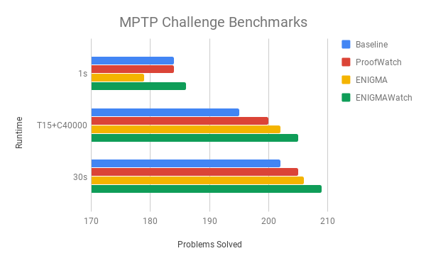
And with appropriate scaling, the immense improvement of our methods over the baseline (except for 1 second) can be seen! Muahahaha :’D
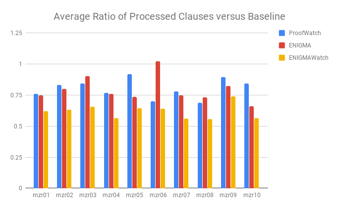
And speaking of odd things, below we have a measurement of “learning on the training set” (usually one uses a training set and a testing set – and maybe a validation set, a fake testing set, too).
The combined ENIGMAWatch indeed cuts down the number of clauses it needs to find its way through the maze. Go figure: taking notes (ProofWatch) when you went through the maze before and then learning how to use these notes helps you do it faster the next time 😋😉.
I found the below experiments interesting (and they didn’t make it into the short paper).
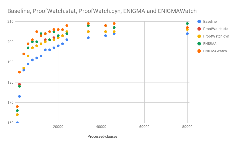
With a high time-limit (60 seconds) I ran the methods with many abstract time limits to see how quickly they learn to prove the same # of theorems.
The initial 20,000 given-clause-loops seem quite important and then progress becomes fairly slow (yet not quite stagnant). This fits the ATP lore I heard from the team that running beyond 1,5, or 10 seconds usually doesn’t help much. Had to see it for myself 🤪
It’s a close race with ENIGMAWatch slightly ahead of ENIGMA.
And the learning ENIGMA is preferred to the “simply mechanistic memory” of ProofWatch.
Back at the time, I had the idea that testing like above is unfair. Why?
Because both ProofWatch and ENIGMA get to learn based off of 1 Baseline run already. So compare them to a \(2x\) Baseline run.
… And ENIGMAWatch learns from 2 Baseline runs. (And this also doesn’t factor in the training time, which is marginal for ProofWatch at least.)
So I multiplied the # of processed clauses by 2 or 3 respectively:
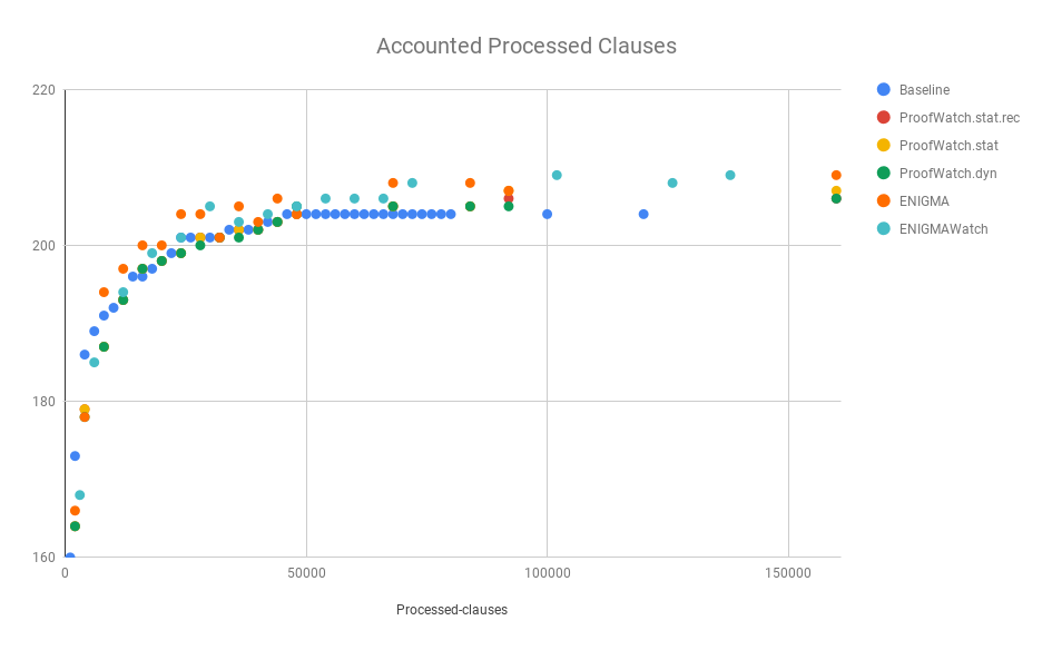
Somewhat surprisingly, ENIGMAWatch catches up without lagging too far behind (despite \(3x\) vs \(2x\)).
And, err, it takes ProofWatch a while to catch up to the Baseline.
After some time passed, I realized it’s silly to try and compare the “accounted run-time” too hard.
Learning is often incremental, and in principle once we learn something, it can be incorporated into the very system and quickly help all future proof-searches.
And the Baseline strategies are the result of a machine learning search as well: they were learned.
And now that we learned, E can benefit from them cheaply.
Currently ENIGMA learns from scratch and ProofWatch has watchlists curated from scratch each time, but this doesn’t have to be the case.
Say a model that can be updated is used for ENIGMA. Then we can help E find a good machine-learned model over proofs of all theorems ATPs have solved. Maybe we want to set aside \(10\%\) as a test or development set for comparing the model to other methods, but in the interest of proving new theorems, it’s best to just keep this model and run with it. We don’t really care so much how hard it was to initially train the all-encompasing ENIGMA model. Because when we have new proofs, new data, we can update the model rather than incurring the full cost. And if your method can’t beat it, just work with it 😉.
We care about the results far more than (small) differences in training time.
We’d brute-force problems (if it actually worked before the Sun went kapoosh).
We’d be happy to run E with simple strategies (if it actually worked and didn’t plateau).
But our little E needs more technic brains to be a happy hungry theorem prover
Next Frontier
The next frontier is to tackle big(ger) data: aim for the full \(57897\) Mizar theorems.
Which, largely, requires a bunch of fun C hacking with sparse vectors and hashing (which my colleague is finishing up now).
And then there’s the question of “how to make watchlist matching faster” to encompass millions of proof clauses. Some sort of hashing or clustering for approximate subsumption?
I have my reservations as to whether it’s actually smart to just dump everything on the watchlist, making all past memories little logic-sensors. But if we can hack the technical side, why not give it a shot and build up (or down (or around)) from there.
To be continued (shortly) . . .